


Objective
Observe and improve the results of running multiple linear regression and random forest algorithms on macroeconomic data to predict currency prices.
Data
- UK, EU and US monthly macroeconomic data for last 20 years was used as the independent variable (X) and average monthly currency price over the same period for GBPUSD and EURUSD was the dependent variable (Y).
- Total no of X variables = 23. Total no of Y values = 219.
- Note that each countries’ macroeconomic data has to be considered separately and US data will impact both currency pairs.
- Core macroeconomic data (interest rate, inflation, GDP, unemployment, etc) that is published monthly was used ignoring the quarterly and annual data.
- The average currency price for each month, Y, was calculated using the End of Day price for each business day in the month (that had published prices) divided by the no of such days.
- Historic macroeconomic data and historic currency prices were taken from our website www.currentiax.com, which sources data from reliable well-known data providers.
Algorithms
- Standard sklearn libraries were used for running the different algorithms in python.
- The data was split into test and training sets, with a test_size = 0.25, as that gave better results compared to 0.2 or 0.33 or other variations.
- Multiple linear regression was used
as the regression algorithm as it gave better results.
- For regression, Backward elimination was used to remove variables with p-value > 0.05, (95% confidence level).
- You can further vary the data using the R-squared value.
- However, difference in results wasn’t significant by varying the p-value or using R-squared value.
- Polynomial regression did not show any useful correlations, with the predicted values having high variance from the test set.
- Random forest gave much better
results with variance between predicted and test sets being much lower compared
to multiple linear regression.
- n_estimators = 20 (number of trees in the forest) gave the best results, any higher or lesser did not improve the results.
Data and Algorithm Logic Variation
- Try changing the number of independent variables (X) considered for regression and random forest using backward elimination to remove X variables with low significance. It gives much better results in some cases, despite not being necessary for random forest.
- Try varying the combination of macroeconomic data for each currency pair. For example, UK, US data impacts GBPUSD, so you can both together or separately to see impact.
- Try varying the time series
considered between the macroeconomic data (independent variable X) and the
average currency price (dependent variable Y). This can be done by creating a time
lag between the two variables.
- I considered Xi vs yi+6m, Xi vs yi+12m and so on.
- Where, i = month in given year and 6m = 6 months lag added to ith month.
- So effectively, we try and use current macroeconomic data to study their impact on future average currency prices, with time lags of 6 months, 12 months, etc.
- This hypothesis is based on the premise that markets are forward looking and start adjusting their view based on future expectations using current data and trend.
- The data and algorithms were used to find out if there is any relation between the macroeconomic data and currency prices. The fact that data with time lag of 12 months gave better results for random forest or multiple regression vs without any time lag, indicates that there is some validity for this hypothesis.
Note – However, this is a very simple premise and by itself not sufficient for all possible variations to the relationship between the macroeconomic data, currency prices and timeframe. There are many other variations that can be tried with the variables, data, time lag, different algorithms used and their parameters. Users can test that on their own and use as they see fit.
Note – The predicted and test results are not an exact match, which is quite difficult for such scenarios and data sets. But the variance is small and reduces further with a larger data size, different time lags and other variables not considered here (central bank monetary policy statements, political statements, etc).
Example Scenario
- As macroeconomic data improves, central banks raise interest rates and tighten monetary policy to counter inflation and a tightening labour market. This can be done at a steady or rapid pace depending on the pace of recovery and growth. Consequently, it results in strengthening or weakening currency, depending on its role in global trade and as a risk-taking currency. This cycle eventually reverses as time progresses and the impact of tighter monetary policy feeds into the economy.
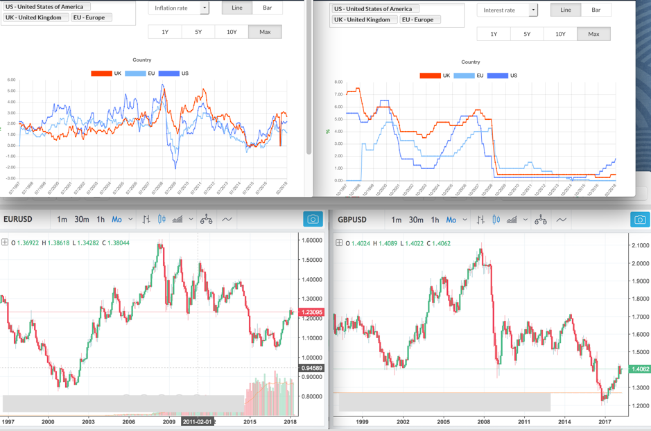
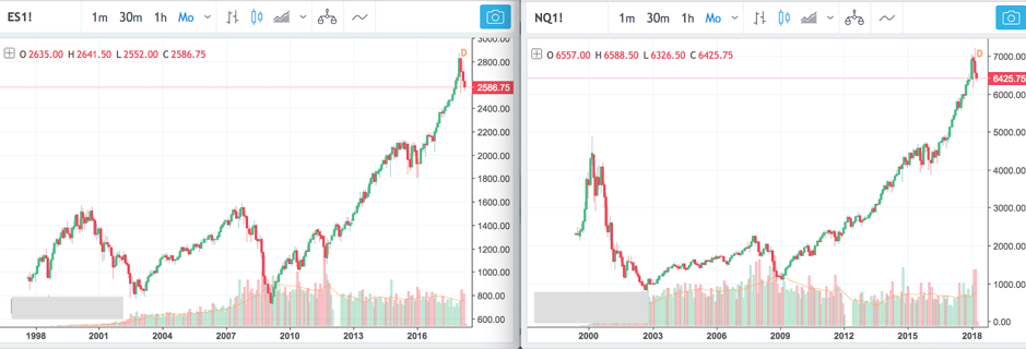
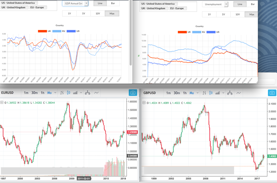
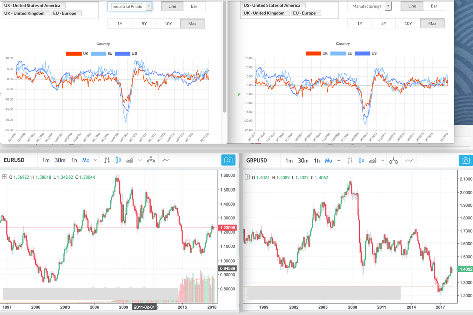
- In the last 20 years we have had 2 big growth and bust cycles (2001 dot-com and 2008 credit crisis) that can be used to validate this. Both have similar characteristics before, during and after the crisis and the macroeconomic and currency data corroborates to that. In fact, major stock market indices have shown very similar up/down cycles and price points during these 2 cycles.
- The charts given at the end of this document show the different macroeconomic data and currency prices for the last 20 years. It shows a clear lag between improving macroeconomic data and impact on currency prices. EURUSD and GBPUSD initially result in a weak USD as the market sees a strengthening economy as an indicator to take on more risk. But at and after the peak of the macroeconomic growth and interest rate cycle, the pattern reverses with USD strength as a move away from risk to safe assets. See the charts for periods around 1998-2003, 2005-2009 and 2010-2018 for macroeconomic data and currency price relationships and repeating patterns.
- However, we can see that indices and other prices post 2010 look highly inflated compared to previous cycles. What is different this time is that the market has been on the rise for a long time without any meaningful reversal. The main reason for this is the amount of monetary easing used by central banks globally to help the economies recover from the throes of a depression on the back of the credit crisis in 2008. It was a necessary and good measure then, but now most global economies or showing very good growth, employment and rising inflation. This has prompted some central banks, especially US, to start unwinding the loose monetary policy by raising interest rates and cutting the Quantitative Easing measures.
- This is a classic cycle of easy monetary policy during crisis/low inflation to return to tighter policy during high inflation/over-heating economy. What is important to consider this time is the amount of asset inflation that has occurred as a result of the cheap money supply.
- This is worrying and indicates that there is a good chance of a big correction in the market. Historic data already indicates that this is a possibility. Combine that with the recent reactions of the market to tighter monetary policy, trade war between major economies like US and China and private debt to GDP back to its high’s in major large economies, indicate the market is increasingly sensitive to negative news. Major indices have failed to breach the high’s in January ’18 after the volatile sell-off in February.
- It might be possible that we have reached the top, though there is still time before interest rates normalize to their long run average and the economic growth momentum is still good. We are not sure how far the trade war will go and its net impact on the economy, which generally impacts inflation due to adjustments in the supply chain.
- Overall, it looks increasingly likely that we are set for a big correction in the market and more volatility. A correction between 40%-80% from the 2018 high’s, depending on the market and inflated valuation, is a possibility and some participants have already started mentioning such scenarios. It would make sense to start considering safer assets, though as usual it is tough to call the top or bottom of the market.
- However, it is important to note that a correction in the market this time doesn’t necessarily imply global economic growth turning to deflation like in 2008. Instead it will primarily be a return to realistic valuations for some highly inflated assets supported by an era of cheap money supply globally.


Sample code and Data
Data used for this analysis along with sample code is given in the below Gitlab location
https://gitlab.com/datawisdomx/currency-price-prediction-macroeconomic-data-regression-random-forest
- Data – macroccyeurusdalldata_3Apr18.csv, macroccygbpusdalldata_3Apr18.csv
- Sample code – MacrodataCurrencyRegressionRandomForest_3Apr18.py
- Results comparison – MacrodataCcyPriceRegressionRandomForestResults_3Apr18.xlsx
Make sure you point the file loader to the correct location of the data file on your local drive. Please get in touch if you see any errors or want to discuss this further at nitin@datawisdomx.com.
Please use them keeping in mind the disclaimer below.
DISCLAIMER – VERY IMPORTANT
The sample data and code are provided only for reference purposes and their accuracy or validity cannot be guaranteed. No guarantees can be made about the accuracy of the data and all data and analysis should be used for reference purposes only. Users should carry out their own data collection, validation and cleaning exercise. Similarly, they should carry out their own analysis by using different algorithms and varying their parameters as they see fit.
Please see the disclaimer page on our website before reading this analysis – https://datawisdomx.com/index.php/disclaimer/


 Algorithms – Results Summary")