


Legal Disclaimer – This research is not an investment advisory or a sales pitch.
Objective
- Predict monthly asset price (main stock indices, commodities, bonds) and direction (Higher/Lower) using macroeconomic data for US, UK and EU by applying regression algorithms
Data
- US, UK and EU monthly main macroeconomic data for last 20 years (Jan 99 – Sep 19) was used for independent variables (X)
- Average monthly high price over the
same period was used for asset prices (main stock indices, commodities, bonds)
as the dependent variable (Y)
- High price was used instead of the close price as it gives the algorithms a wider range (peaks) to make predictions with and reduces known range/averaging bias
- All 3 countries’ macroeconomic data was combined to see their impact on asset prices
- Historic Asset price data has been sourced from public data sets. Macroeconomic data was taken from our website https://datawisdomx.com, which sources data from reliable well-known data providers
Algorithms
- Standard python scikit-learn, pandas, numpy, visualization libraries were used for running the different algorithms in python
- Regression algorithms used – Random Forest, Support Vector Machine, Multiple Linear and XGBoost
- The data was split into test and training sets, with a test_size = 0.25, as that gave better results compared to 0.2 or 0.33 or other variations.
- Feature scaling – Data wasn’t
standardized as it would require the new independent data vector for new price prediction
to be standardized using the trained models mean/variance
- This is not ideal as it would standardize the new independent data vector using old mean/variance of the trained model, distorting its real impact on the predicted value
- Also, with Random Forest/XGBoost algorithms it’s not necessary as they are based on decision tree ensemble model (Bagging/Boosting), which does not require standardization (not distance based)
- Metrics used for
evaluating the algorithms were
- MSE – Mean Squared Error, RMSE – Root Mean Squared Error
- MAE – Mean Absolute Error
- R2 – R-squared
- Model
training/testing, prediction and validation logic
- Model – Yt = F(Xt-1), where Y – Asset Price vector (Dependent variable), X – Macroeconomic data vector (Independent variables)
- Prediction – Previous months’ (t-1) macroeconomic data (X) is used to predict
next months’ (t) asset price (Y). ‘t’ is the current calendar month
- Eg: Trained model uses August (t-1) macroeconomic data to predict September (t) asset price
- Training/Testing – Model is trained/tested with data (X, Y) up to the previous month
(t-1). Train/Test split of 0.25 was used
- Independent variable data needs to be updated regularly during the month as latest macroeconomic data becomes available
- It will also require retraining of the model for each update
- Till the latest value becomes available, last months’ value (or most recent) will be used for retraining
- Validation – Validation results are given for the last 3 months for S&P500, DAX, Gold, WTIOil,
USTreasury10Year bond price
- The validation data (independent and dependent data vectors) was removed from the sample data set so that it’s not used for training/testing the model (prevent leakage)
- Model was trained/tested with and without time lag
- Time lags considered were 6 and 12 months
- Hyper
parameter tuning – was done using GridSearchCV
- It also ensures that multiple variations of the data sample are used by shuffling it randomly for k-fold splits, thereby preventing overfitting on the same test data and reducing bias
- Below hyper parameters gave the best results
- XGBoost – ‘rgr__learning_rate’: 0.1, ‘rgr__max_depth’: 4, ‘rgr__seed’: 1
- RandomForest – n_estimators=500, criterion=’mse’, min_samples_leaf=2, max_depth=15, min_samples_split=2, max_features=’sqrt’, random_state=42, n_jobs=-1
- Python code for data wrangling, GridsearchCV hyperparameter tuning for each model, model explanation details for Random Forest and XGBoost and data visualization is given in github – AssetPriceDirectionMacroData_22Oct19.py
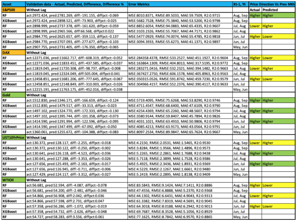
Results Analysis – Without Time Lag
- Results are average/variable as predicted price is consistently below actual price, irrespective of asset type and its date in the series
- Also, predicted asset price direction for
validation data is not consistent for all asset types
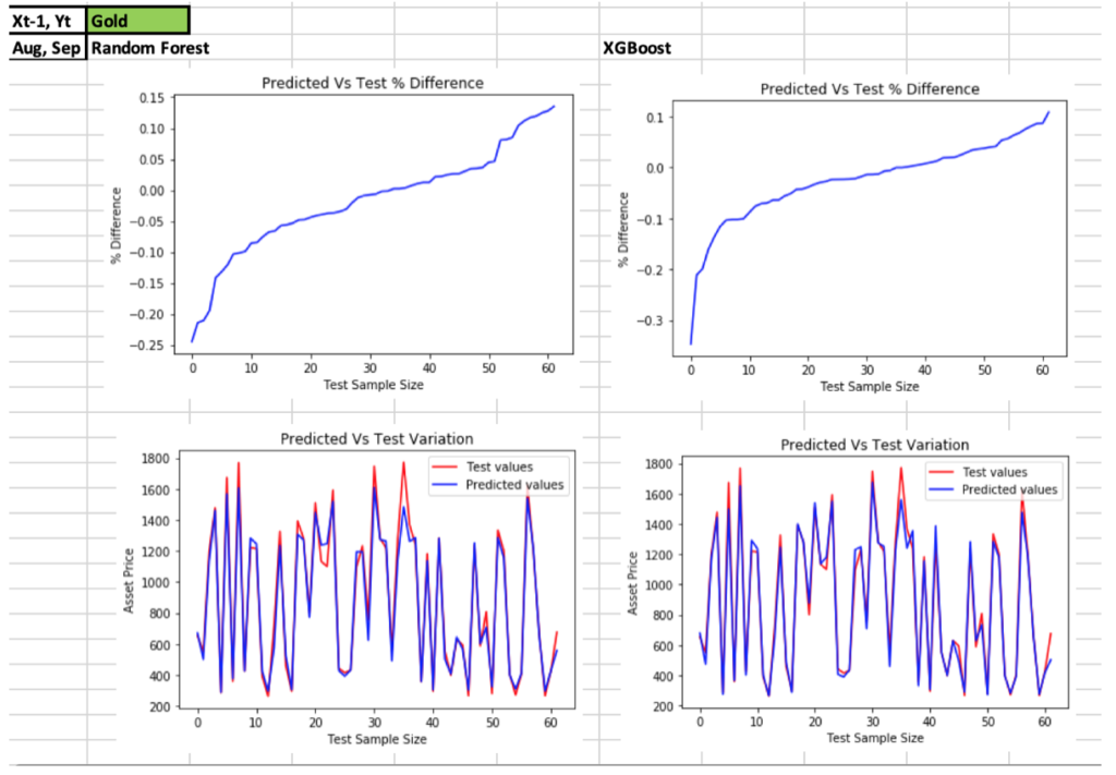
- Gold, USTreasury 10 Year Price – Directionally, predicted asset prices are correct relative to actual
- Equities, Oil – Directionally, not giving a consistent result. Opposite of actual
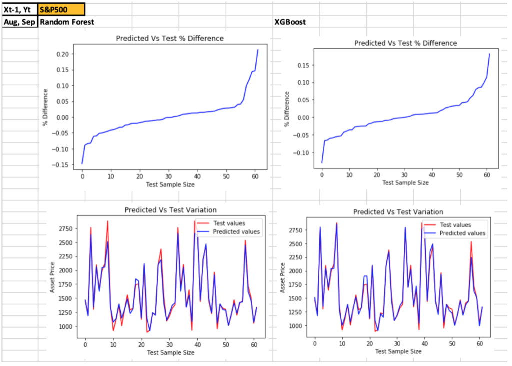
- Comparing predicted asset prices with test prices – More than 75% of the predicted values were within a +/- 5% difference from the test values, depending on the asset type
- XGBoost gave the best results in terms of
lower MSE, RMSE, MAE and higher R-squared values indicating higher accuracy and
closer prediction (goodness of fit)
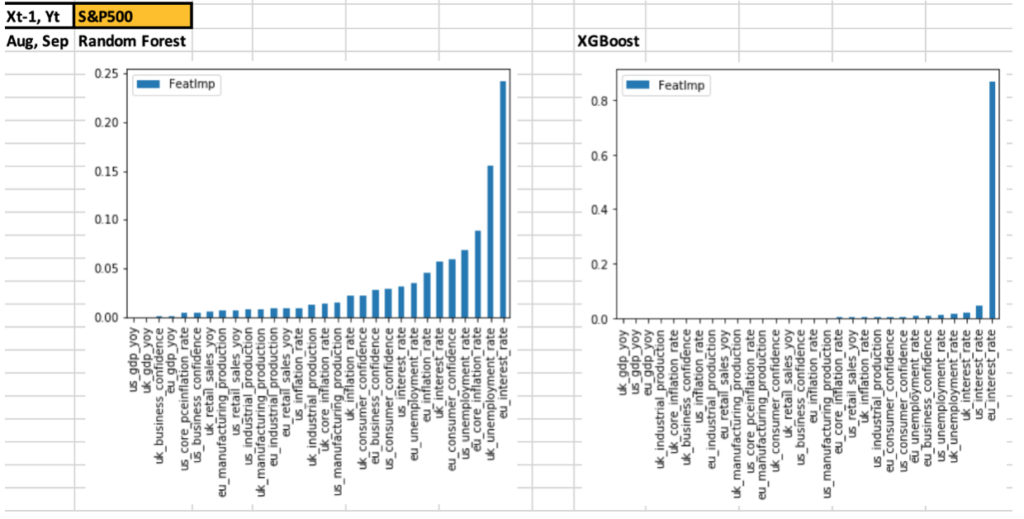
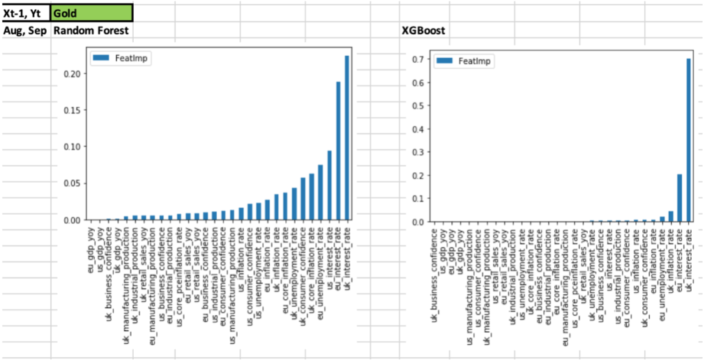
- However, it’s giving very high importance to one feature and low to the rest
- Stock indices – eu interest rate
- Gold – uk interest rate
- US10YrTreasury Price – uk, eu interest rate
- WTIOil – us consumer confidence, uk inflation rate
- This looks like over-fitting as asset prices are dependent on a variety of macroeconomic data with varying importance
- However, it’s giving very high importance to one feature and low to the rest
- Random
Forest gave slightly worse results than XGBoost, but
the feature selection is
more varied and covers a wider range
- Common features from all
3 countries – EU/UK/US
- Interest rate, inflation rate, unemployment rate, consumer confidence
- This looks like a more realistic result and is preferred compared to XGBoost
- Common features from all
3 countries – EU/UK/US
- Results are given in the spreadsheet
– AssetPriceDirectionMacroDataResults_22Oct19
- Predicted vs actual results are given for – S&P500, DAX, Gold, WTIOil, USTreasury10Year price
- Results are given for Random Forest and XGBoost algorithms
- It
contains the evaluation metrics, predicted vs actual value for validation data
- Validation results are given for the last 3 months (Jul-Sep) of 2019
- Code and data are given for other asset types and algorithms. Users can use them to back test historic variations
- Result grid for predicted vs actual price & direction and evaluation metrics is given below
- Feature importance charts for both algorithms and all assets are given in the spreadsheet
- Given below is a sample of the charts for S&P500 and Gold for both algorithms
- Predicted
asset prices vs test prices charts for both algorithms and all assets are given in the spreadsheet
- Given below is a sample of the charts for S&P500 and Gold for both algorithms
Results Analysis – With Time Lag (6, 12 months)
- Results are worse than without lag. Not considered
Further research, ways to improve algorithms
- This
is a good starting point as the model can now be improved by
- Further analysis to bring predicted price closer to actual price
- Further analysis to determine better approach for equities and oil price direction
- Adding other data types (central bank statements, political statements, etc) and other countries’ data (China, India, Japan, etc) can improve the results, as they are relevant
- Create algorithm to consider the cumulative impact of all data types, rather than raw features
- Another way to
cross-check and improve the results would be to combine the results of both algorithms
(ensemble technique) and then take a decision
- This might be possible as both Random Forest and XGBoost are based on decision trees, though with different ensemble approaches
- It’s possible to run both algorithms in parallel and take a decision when both confirm the same direction
- Use dimensionality reduction like PCA to see if it improves the results, though it reduces explainability
Conclusion
- While the results are average/variable, they still show validity for some asset types directionally
- As all possible data has not been considered, this was expected
- As other data types and more samples are included, expectation is that it will improve the results
- Results further validate prior research on correlation between asset prices and macroeconomic data
- It provides a good base to work with to improve the results
Sample code, Data and Results
Data & sample code used for this analysis along with results & summary are given in the below Github location –
https://github.com/datawisdomx/Predict-Monthly-Asset-Price-and-Direction-using-Macroeconomic-Data
Published research – Asset price/Macroeconomic data relationship and Market Analysis
- Results of this new research further
validate earlier research article already published on github
- It shows the correlation and coefficient of determination relationship between them
- The macroeconomic factors which had the highest correlation are also amongst the most important features for the pricing algorithms, especially random forest
- https://github.com/datawisdomx/Monthly-Asset-price-relationship-to-Macroeconomic-Data
Note – This research is based on a very simple premise and small data set. This by itself is not sufficient for all possible variations to the relationship between macroeconomic data, countries, asset prices, timeframes, algorithms used and other factors like political & central bank data, etc. Users can test that on their own and use as they see fit.
Disclaimer
Please use this research keeping in mind the disclaimer below.
Please get in touch if you see any errors or want to discuss this further at nitin@datawisdomx.com


 Algorithms – Results Summary")


