Regression- Types, Metrics, Comparison via Pipeline GridSearchCV

This article will discuss the basic theory and relevant code examples for different regression algorithms. It will also show how to test and compare multiple regression algorithms at once on the same dataset, to find the best fit algorithm, using Pipeline and GridSearchCV.

The regression algorithms considered are

• Multiple Linear Regression
• Regularization – L1 Lasso and L2 Ridge
• Random Forest Regression
• XGBoost Regression

Code for different algorithms and data used are given in github.

Note – Make sure to point the code to the right directory in your setup

https://github.com/datawisdomx/DataScienceCourse/tree/main/Part1-MachineLearningandDataAnalytics/Examples/Chapter8_Regression

https://github.com/datawisdomx/DataScienceCourse/tree/main/Part1-MachineLearningandDataAnalytics/Data

Regression algorithms are used for predicting values on a continuous scale (real numbers, not just 0 or 1 categories)

• Dependent variable Y values (target function) are predicted using the independent variables X_1..n (features)
• Common types are Linear, Multiple linear, Random Forest, XGBoost, Neural Networks, etc
• Regression concepts are given below briefly:
• Regression is a statistical process for estimating the relationship between a dependent variable Y and one or more independent variables X_1..n in a sample
• 
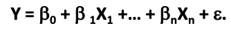
• B – unknown parameters (coefficient) for each X. e – deviation error of sample values from actuals
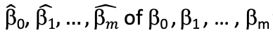
• The goal is to estimate a function Y ̂ that closely fits the data.
• 
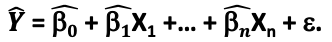
• B ̂ is the estimate of each parameter
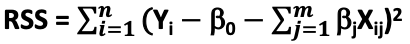
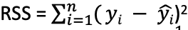
• Models like Ordinary Least Squares OLS estimate B ̂ by minimizing the loss function Residual Sum of Squares (RSS)
• OLS = Min (RSS)
• RSS =
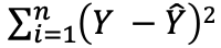
• Effectively, the model tries to minimise the difference between the predicted and actual values (best fit line)
• The model uses error metrics like MSE, RMSE, MAE, R² for minimizing the loss function
• Geometrically it is the sum of the squared perpendicular distance of each sample point from the best fit line passing through them
• Closer the points are to the line, better the fit Useful website – https://scikit-learn.org/stable/modules/linear_model.html

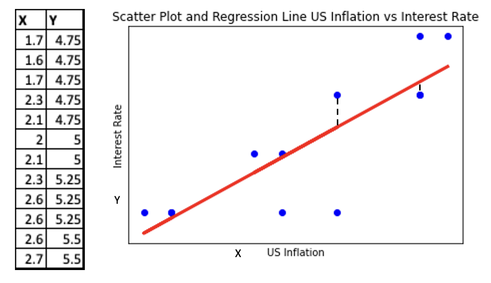
Consider a simple linear model between

• Inflation (X) and Interest rate (Y)
• US economy monthly data is given for 1999
• We know that Interest rate is normally increased when inflation increases
• Scatter plot is shown of actual values Y_i (blue dots), with the predicted values (Y_i^{^})  on the best fit regression line (red) through them
• The model minimises the sum of the vertical distance between all points Y_i (x_i,y_i) and (Y_i^{^}) on the best fit line
• For a simple 2 variable sample, it can be represented as the equation of a straight line Y = mX + c
• m – slope of the line, c – y-intercept  (x=0)

Multiple Linear regression

• It uses a linear equation of multiple independent variables (X_1…m) to estimate the relationship with the dependent variable Y
• The relationship between Y and each X_1…m is linear
• So, Y is now a linear equation of multiple independent X variables (X_1, X_2,…, X_m)
• For a multiple linear function of X, equation for Y becomes
  • 
• i = 1 … n is the no of rows of sample data, j = 1 … m is the no of independent X variables
• Ordinary Least Squares method finds that minimizes the sum of the squared errors e (RSS)
  • 
• Equation of the best fit regression line will be
  • 
• Sklearn.Linear_model, LinearRegression library is used for building a multiple linear regression model
• The sample of Bond Prices (Y) and Inflation rate (X), used in the linear model is further enriched by adding other data
• US macroeconomic factors that impact bond prices like consumer confidence, retail sales, industrial production and unemployment rate
• This is true for most real-world problems, where the output variable’s value depends on multiple input variables
• The multiple linear regression results further improve on the results of the single independent variable linear model for predicting Bond Prices (Y)
• This occurs as with more variables and data the estimator can learn more about the model resulting in better predictions
• However, the results are still not accurate enough
• Note – It is important to note that just getting better metrics does not mean better predictions, as error terms like MSE and RMSE can degrade due to a few outlier values

Polynomial regression

• Uses linear regression to fit polynomials to the data.
• But has not been discussed as it is not useful for this example. It can easily be implemented
• It uses linear algebraic equations of the n^th degree to estimate the unknown parameters B ̂_i
• 

Regularization regression

• Is the process of adding a small amount of bias to a linear regression model to induce smoothness in order to prevent overfitting (complexity)
• This is done by adding a penalty term λ to the loss function RSS which penalizes increase in the unknown parameters B
• Ridge regression or L2 regularization
  • It modifies the loss function RSS by adding the penalty term λ which is a square function of the unknown parameters “B”
  • 
  • Ridge regression loss function =
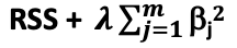
  • λ penalizes increase in “B” parameters in order to minimize the modified loss function
  • λ = 0 makes it a linear model. As λ -> ∞, “B” -> 0, increasing the penalty
  • This is how Ridge regression keeps the “B” parameters small
  • However, as “B” parameters are never equal to 0 all features will be selected, even insignificant one’s
• Lasso regression or L1 regularization is similar to ridge regression except that the penalty term λ is a modulus function of the unknown parameters “B”
  • Lasso regression loss function =  RSS +
  • For a large λ some of the parameters can be 0, so it also enables feature selection, improving interpretability
  • Regularization can reduce the variance without significantly increasing bias, but only up to a limit
  • So, the right value of λ has to be selected
• We’ll use the same data for predicting US 10 year govt Bond Prices (Y) using multiple US macroeconomic variables (X_1…n)
• The results are similar to multiple linear regression but they are still not accurate enough

Decision trees

• Are not discussed in detail as its more advanced versions – RandomForest and XGBoost are more widely used
• Use a hierarchical tree-based structure with parent and child nodes connected by branches (conditions)
• They split the sample dataset into different subsets (branches) based on the result of conditions
• Decision tree builds a model Y = f(X_1…n) that minimises Information Gain and optimizes Gini Impurity to 1

Ensemble algorithms

• Combine the predictions of several estimators (weak learners), generally the same algorithm, to give a result better than using a single estimator
• Two main ensemble methods are – bagging and boosting
• Bagging (Bootstrap aggregating) applies the same estimator to independent subsets of the sample, training them in parallel and takes the average of their predictions to build an ensemble that give better results with reduced variance. Eg: Random Forest
• Boosting builds the ensemble sequentially by applying the same estimator iteratively to the entire dataset, each time reducing the errors of the previous iteration and adding the new predictions to the previous iteration. It gives results with reduced bias. Eg: Adaboost (Adaptive Boosting), GradientBoost, XGBoost

Random Forest

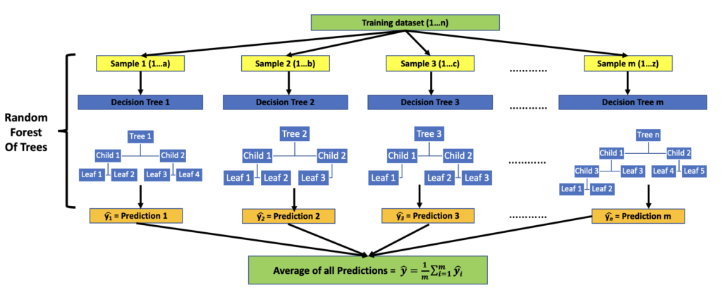
• It is an ensemble of decision tree estimators that trains multiple estimators in parallel on subsets of the dataset and then averages their predictions to reduce errors and get the best results
• Each tree is built from a random sample drawn with replacement from the training set (bootstrap sample)
• Training set – 1…n, Decision Trees – 1…m. m < n
• Sample 1 – 1…a, where a < n. Similarly, Samples 2,3 … m
• It is a random forest of decision trees (tree nodes, splitting, children, leaves)
• Random forest builds a model Y = f(X_1…n) that minimises Information Gain and optimizes Gini Impurity to 1
• Y – Dependent variable, X_1…n – Independent variables
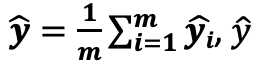• – is the average of all predictions, (y_i) ̂ is the prediction of each decision tree i
• Output y ̂ is a real number
• Randomness is introduced in the ensemble by the sampling technique and other parameters like number of features used for splitting and tree depth
• Random forest model reduces the estimator variance by averaging the results of multiple decision tree estimators
• RandomForest model is good for interpretation as it has a feature_importances_ attribute that gives a relative importance to each feature (X) with values between 0 and 1, total of all values being 1
  • Higher value indicates higher importance of feature in determining Y
• Example of how a RandomForest model is trained on the dataset is given below

XGBoost (Extreme Gradient Boosting)

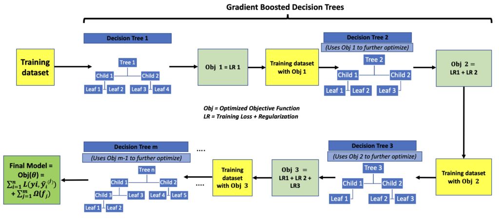
• It uses gradient boosted decision trees, adding a new tree sequentially in each iteration to optimize the Objective function
• It consists of a Training Loss function L(θ) and a Regularization term Ω(θ)
• Obj(θ) = L(θ) + Ω(θ)
• θ – parameters of the model we learn from the data
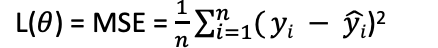
• Training Loss function L(θ) is a prediction accuracy measure (predicted-actual) like MSE
• 
• Regularization term Ω(θ) controls model complexity by reducing overfitting to the data (using bias-variance tradeoff)
• XGBoost uses an additive strategy by fixing the previous iteration’s errors in the next iteration by adding a new tree
• It does not use a traditional gradient descent algorithm by calculating the gradient (convex curve, where loss function goes down/up the slope to minimize the loss)
• XGBoost builds a model Y = f(X_1…n) that optimizes the objective function Obj(θ)
• Y – Dependent variable, X_1…n – Independent variables
• Training set – 1…n, Decision Trees – 1…m. m < n.
• y_i – actual values, (y_i^{^}) – predicted values, (y_j^{^}) – prediction of each decision tree
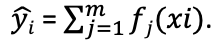• . Training data i = 1…n, No of trees j = 1…m. m < n.
• 
• (y_i) ̂^(j) – is the prediction value for tree j
• It is the most popular implementation of gradient boosting for both accuracy and speed
  • It does not train multiple trees in parallel like random forest
  • It does parallel processing within each tree by building each branch in parallel
  • It performs in memory sorting and splitting of all features once in parallel, which are then stored and reused again
• XGboost model is good for interpretation as it has a feature_importances_ attribute that gives a relative importance to each feature (X) with values between 0 and 1, total of all values being 1
  • Higher value indicates higher importance of feature in determining Y
• Example of how a XGBoost model is trained on the dataset is given below
• Useful website – https://xgboost.readthedocs.io/en/latest/tutorials/model.html

Regression – Error Metrics

• To choose the best estimator (model) we use error metrics like MSE, RMSE, MAE, R²
• MSE – Mean Squared Error is the average of the sum of squares of the errors (predicted-actual values)
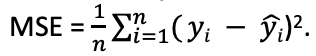  • . y_i – actual value. (y_i^{^}) – predicted value
  • We want to minimize MSE. Closer it is to 0, better the estimate
  • It penalizes even the smallest error due to the squaring
• RMSE – Root Mean Squared Error is the square root of MSE. It is the preferred metric as it has the same unit as the data
  • 
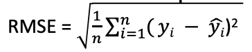
  • We want to minimize RMSE. Closer it is to 0, better the estimate
  • It penalizes large errors
• MAE – Mean Absolute Error is the average of the absolute difference between predicted and actual values
  • 
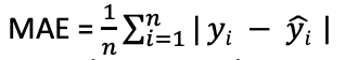
  • It is robust to outliers as it weighs all differences equally. Not useful if you want to identify outliers
• R² (Coefficient of Determination or Goodness of Fit) –  It explains how well the model fits the sample
  • It is the proportion of variance in the dependent variable that is predictable from the independent variables
  • R² = 1-(RSS/TSS)
  • Sum of Squares of Residuals,
  • Variance of the model’s predictions. Regression minimizes RSS
  • Total Sum of squares,
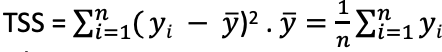
  • Variance of the dependent variable
  • Closer it is to 1, better the estimate
• Useful website – https://scikit-learn.org/stable/modules/model_evaluation.html#regression-metrics

Pipeline and GridSearchCV

• Now we will see how to use these libraries to build, optimize and evaluate multiple regression algorithms at once and then select the best one
• Pipeline combines data transformations and training multiple models into a sequence of steps
• Grid search across entire hyperparameter grid to select the best combination for each model
• Hyperparameters to be tuned for each model are setup as a predefined parameter array (grid)
• GridSearchCV performs k-fold cross-validation to train models on multiple variations of the training data of the sample in an iterative loop (k-folds, k-splits)
• The results of applying GridSearchCV algorithm on a pipeline of different regression models to predict US bond prices using US macroeconomic data are shown
• The regression algorithms considered are
  • Multiple Linear Regression
  • Regularization – L1 Lasso and L2 Ridge
  • Random Forest Regression
  • XGBoost Regression
• A 10-fold cross-validation splitting strategy is used to ensure multiple variations of the training data are used (better data sampling)
• Sklearn_metrics are used to evaluate and measure the accuracy of the results
• The results are better for all models
  • The hyper-tuned parameters can now be used for each model
• Random Forest and XGBoost still give the best results compared to all other models
• Useful websites are:

https://scikit-learn.org/stable/modules/cross_validation.html

https://scikit-learn.org/stable/modules/grid_search.html

https://scikit-learn.org/stable/modules/compose.htm

Giving the code for Pipeline and GridSearchCV here as it shows how easy it is to try different regression models with hyperparameter tuning with just over 100 lines of code.