Classification- Types, Metrics and Comparison via Pipeline GridSearchCV

This article will discuss the basic theory and relevant code examples for different classification algorithms. It will also show how to test and compare multiple classification algorithms at once on the same dataset, to find the best fit algorithm, using Pipeline and GridSearchCV.

Code for different algorithms and data used are given in github.

Note – Make sure to point the code to the right directory in your setup

https://github.com/datawisdomx/DataScienceCourse/tree/main/Part1-MachineLearningandDataAnalytics/Examples/Chapter9_Classification

https://github.com/datawisdomx/DataScienceCourse/tree/main/Part1-MachineLearningandDataAnalytics/Data

Classification algorithms are used for predicting a class or category. It is used for predicting discrete values or classes instead of continuous values.

Classification is generally of 2 types:

• Binary – Data is categorized into one of 2 classes (0 or 1, ‘True’ or ‘False’, etc)
• Multiclass – Data is categorized into on of the many classes (0,1,2,3; ‘City1’, ‘City2’, ‘City3’, etc)

Some common examples for classification are:

• Assign 0 or 1 to each observation based on a condition being true or false
• Assigning each email  to ‘spam’, ‘not spam’ category by using prior spam email data
• Detecting the ‘presence’ or ‘absence’ of a disease by using prior disease symptom data

Popular classifiers are Logistic regression, K-Nearest Neighbours (K-NN), Support Vector Machines (SVM), Naïve Bayes, Decision Trees, Neural Networks, etc

Classifiers use error metrics like confusion matrix (True/False Positives/Negatives), ROC curve, etc

As all machine learning classifiers work with numbers and since the data can be numeric (integer or real), ordinal (‘true’, ‘false’) and categorical (text like city, group type, etc), it needs to be transformed. As most classifiers are similarity or distance based, they generally require standardization (scaling).

Sample data used for classification problems is described below:

Binary

• https://data.world/exercises/logistic-regression-exercise-1
• Dataset for practicing classification -use NBA rookie stats to predict if player will last 5 years in league
• Classification Exercise: Predict 5-Year Career Longevity for NBA Rookies
• y = 0 if career years played < 5
  y = 1 if career years played >= 5

Multiclass

• https://www.kaggle.com/scarecrow2020/tech-students-profile-prediction
• Tortuga Code is an online educational platform, oriented over programming and technology
• Tortuga Code is looking for a recommender system that assigns students to a specific category depending on their developer profile.
• Multiclass Classification: Predict student developer category

Error Metrics

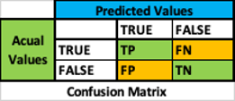
• A Confusion matrix is used to evaluate the accuracy of a classifier, as we need to know how many values are predicted correctly for each class label
  • Rather than a single measure of accuracy or error
• A NxN table is used to summarize the results of the confusion matrix. N is the no of classes in the classifier
  • Each row represents values in the actual class
  • Each column represents values in the predicted class
  • The table cells contain the count of class labels that are predicted correctly or incorrectly
• For example, a binary classifier has a 2×2 table matrix
  • True, False representing 1, 0 class labels for Y
• Using the predicted and actual class values, the row/column intersection represents the count of values that are called
  • True Positives (TP) – Predicted True, Actual True
  • True Negatives (TN) – Predicted False, Actual False
  • False Positives (FP) – Predicted True but Actual False – Type 1 error
  • False Negatives (FN) – Predicted False but Actual True – Type 2 error
  • Type 1, Type 2 error importance depends on the problem (disease, fraud, etc)
• Other measures of accuracy are
  • Accuracy rate = Correct predictions (TP+TN) / Total predictions
  • Error rate = 1 – Accuracy Rate
  • Precision = TP / (TP+FP). What ratio of correctly predicted values are true
  • Sensitivity or Recall or True Positive Rate TPR = TP / (TP+FN). What ratio of actual true values are correctly predicted
  • False Negative Rate FNR = FN / (TP+FN). What ratio of actual true values are incorrectly predicted
  • A high TPR and low FNR means more correctly predicted true values
  • Specificity or True Negative Rate TNR = TN / (TN+FP). What ratio of actual false values are correctly predicted
  • False Positive Rate FPR = FP / (TN+FP) = 1-Specifity. What ratio of actual false values are incorrectly predicted
  • A high TNR and low FPR means more correctly predicted false values

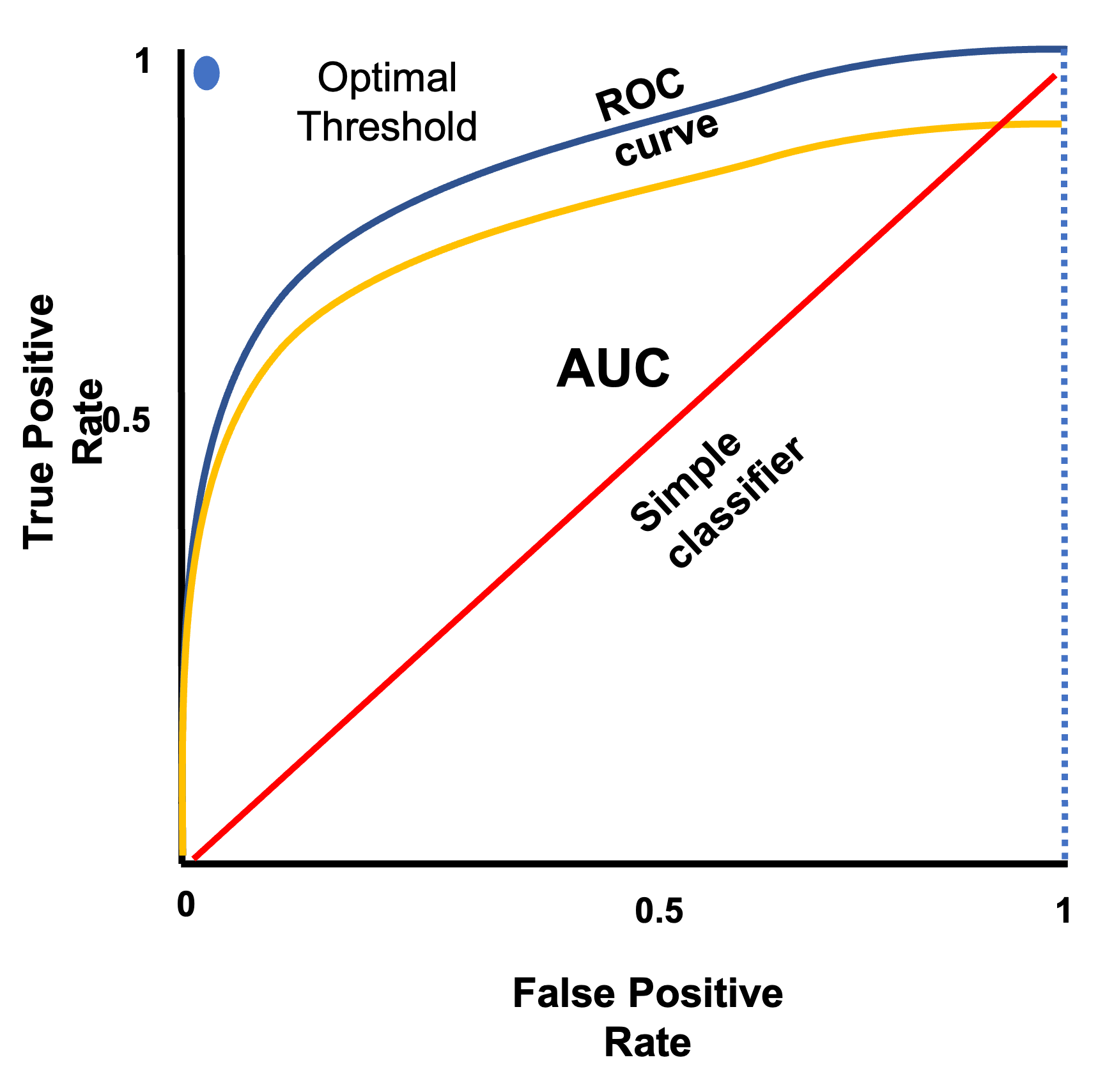
ROC (Receiver Operating Characteristic) curve is used for evaluating binary classifiers

• It is a probability plot of True Positive Rate against False Positive Rate for different threshold values
• It is a plot of sensitivity vs 1-specifity, indicating how sensitive the classifier is to false positives
• It is used for selecting the optimal model by varying the decision threshold value used by the classifier
• It is used for cost-benefit analysis when selecting the optimal decision threshold
• The steepness of a ROC curve is increased to maximize the true positive rate while minimizing the false positive rate
• The top left corner of the plot is the ‘optimal threshold’ where TPR = 1 and FPR = 0
• This means all true and false values are correctly classified (no false positives)
• AUC curve – is the Area Under the ROC Curve
  • It is the probability that the classifier ranks true values higher than false values. It is a summary of the ROC curve
  • AUC varies from 0 to 1. The larger the area under the curve the better the classifier
• 

Logistic Regression

• It is a linear model for classification problems
  • Not a regression model despite its name
• It builds a logistic model that assumes a linear relationship between the probability of the log-odds of the dependent variable Y (output class label) and the Independent variables X_1…n (input)
  • The class labels are distinct values – 0,1 for binary or 0,1,2…n for multiclass classification
• The logistic model estimates the class label of Y by
  • First using a logistic function to calculate the probability of the log-odds of Y varying between (0,1)
  • Then using a decision threshold to convert the probability between (0,1) into a distinct class label (0,1,2, etc)
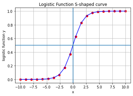
• A logistic function (sigmoid function) is an S-shaped curve, with real number inputs between (-∞, +∞) and output probability between (0,1)
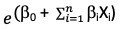
  • The equation for a standard logistic function f(y) = 1 /(1 +e^-y), e is the exponential function (growth/decay)
• A plot of a simple logistic function f(y) for x between  (-10, 10) is shown

To understand this, consider a binary classification problem where Y is either 0 or 1

• Y = 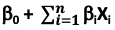 is a linear regression equation for Y dependent on multiple independent variables X_1…n
• P(Y=1|X) = p = probability of the dependent variable Y=1 occurring, given X independent variables
• A logit function, which is the inverse of a logistic function, is used to derive the logistic regression equation
• It is used to calculate the log-odds of the probability by taking the logarithm of the odds of the probability
• Given p, Odds = p/(1-p) = (“event happening”  (Y=1))/(“event not happening”  (Y=0))
• So, Logit(p) =  log_e((p/(1-p)) )
• Normally natural logarithm e is used but it can be any base (2, 10, etc)
• As the log-odds of the probability is assumed to be equal to a linear function, log_e((p/(1-p)) ) =
• By using exponential function, we can transform logit(p) to get p/(1-p) =
• Applying algebra, we get p = 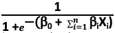= f(y), a logistic function of a regression equation
• p is the probability varying between (0,1)
• b – the unknown regression coefficients will be estimated using maximum likelihood estimation (covered later)
• Conclusion – This shows that while the linear regression equation (input) can vary from (-∞, +∞), probability p (output) varies between (0,1) being the result of a logistic function of a linear regression equation

Now, using a decision threshold (cut-off) on the probability p the logistic regression model assigns a discrete value of 0 or 1 as a class label for Y

• Eg: If p >= 0.5, class label = 1. Else class label = 0
  • 0.5 is the default threshold for binary classification
  • However, the threshold value can be optimized to get the best threshold for class labels
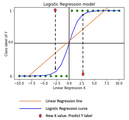
• Logistic regression model graph for X (-10,10) is shown
• Comparing logistic regression to linear regression, the model converts a non-fitting straight line into a best fit S-shaped line
• We can now predict the class label for new X values depending on where they fall on the best fit logistic model curve
• The benefit of using a logistic regression model is that it improves interpretability by transforming large changes in X into a smaller range for Y
  • While the odds increase exponentially (for a unit increase in X and b, the odds increase by e^BX)
  • As Odds =
  • The log-odds increase at a constant rate (logarithmic function)
  • Causing only a small increase in probability p

Logistic Regression can be used for multiclass classification by using the ‘one-vs-rest’ or ‘one-vs-all’ strategy

• ‘one-vs-rest’ trains a single classifier per class, with the samples of that class labelled as 1 and all other samples as 0
• It is preferred for multiclass classification

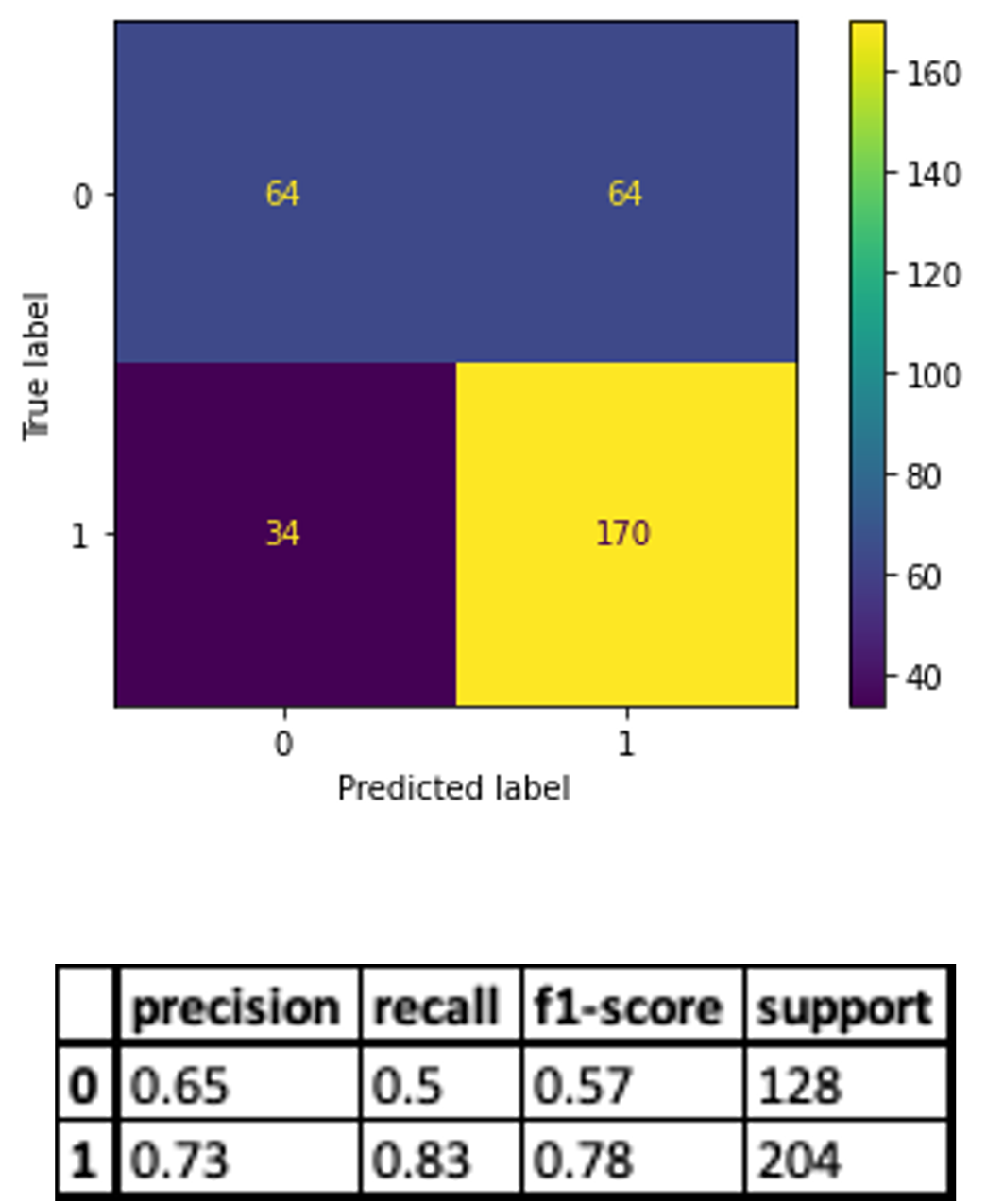
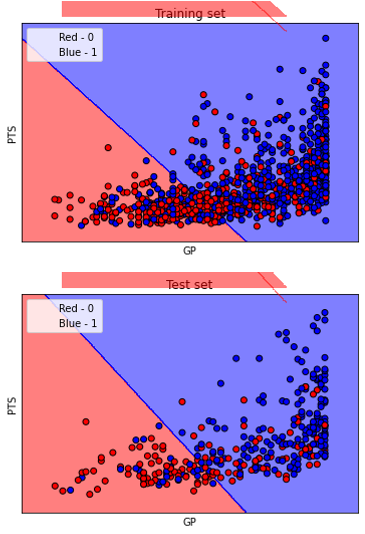
The results of the algorithm on the NBA rookie stats to predict if a player will last 5 years in league show good results (~ 72%)

Confusion matrix, classification report and scatter plot of the results with a best fit decision boundary are given

• 
• 

K-Nearest Neighbors

• It is an instance-based non-parametric classifier
  • It does not involve estimation of parameters to build a model using training data
  • It does not make any assumptions about the model function Y = f(X_1…n), between the dependent variable Y (output class label) and the Independent variables X_1…n (inputs)
  • It is a non-linear classification model
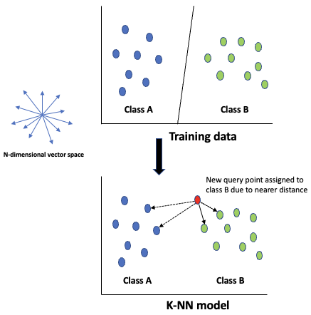
• It stores in memory instances of all training data as n-dimensional vectors in a multidimensional feature space, with labelled classes
  • Each observation is represented as a vector of independent variables (X_1…n)
  • It uses fast indexing structures like KDTree or Ball tree to overcome speed and memory issues due to large instances of the training data
• A Class label is assigned to an unlabeled observation (query point) based on a simple majority vote of the nearest neighbors (most common class in k neighbors nearest to it)
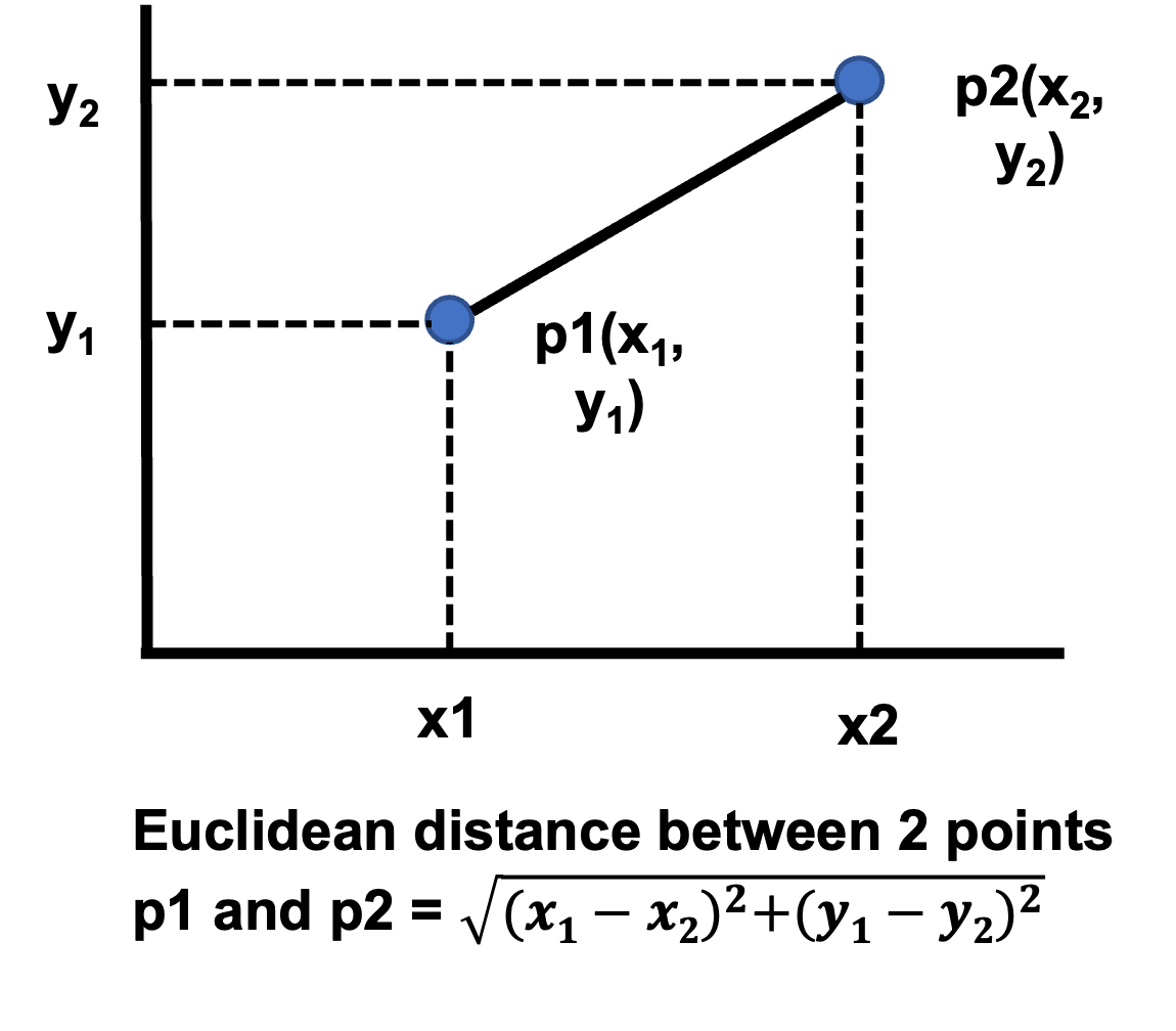
• It uses Euclidean distance to calculate nearness of the query point to its k neighbors
  • k is a user defined integer. Optimized using hyperparameter tuning
  • Higher k value reduces the impact of noise
  • Normally same weight is assigned to each neighbor of the query point
  • Sometimes higher weight is assigned to nearer neighbors by using the inverse of distance from the query point to get a better fit
• 

• Being distance based it requires standardization (scaling) of data to prevent giving higher weight to independent variables with larger scales
• It is useful for problems where the decision boundary is irregular (not separable by a linear hyperplane)
• Algorithms used to calculate the distance are:
• Brute force – Euclidean distance is calculated between all pairs of points. Inefficient for large sample sizes
• KD Tree (K dimensional tree) –  It reduces number of distance calculations by encoding aggregate distance information
• Ball Tree – Better for higher dimensions. Recursively partitions the data into a series of nested hyper-spheres
• 

Support Vector Machines (SVM)

• Used for classification by building a hyperplane that best separates the labelled classes in the training data
• For labelled training data with n-features (independent variables (X_1…n)), each observation is represented as a vector of n-dimensions in the feature space
  • Each observation is a point with n-dimensions (value of each feature)
• A new observation can be classified into the correct class using the hyperplane
  • There can be multiple hyperplanes that separate the classes, but the model selects the best one using different optimization techniques
  • Eg: For binary classification with 2 classes, the hyperplane will be a single line
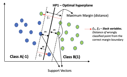
• The SVM classifier (SVC) finds the best fit (optimal) hyperplane by calculating the largest distance (maximum margin) between points of the different classes nearest to the hyperplane
• These points are called support vectors (margin boundaries), being most unlike the class they are in
• Larger the margin, farther away are the boundary points from the hyperplane
  • The more these points are like the class they are in and less like the other class
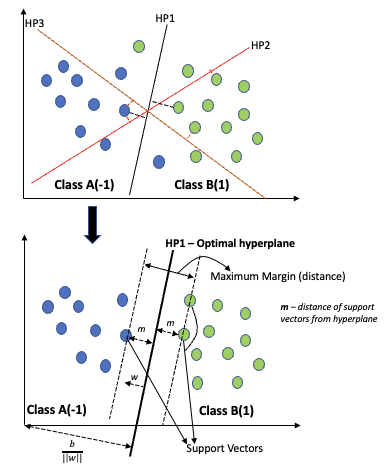
• Consider a binary classification problem with 2 classes (A,B) labelled (1,-1) that can be separated by many hyperplanes (HP1, HP2, HP3, etc)
  • For HP2 and HP3, the support vectors are very close to the hyperplane resulting in a small maximum margin
  • HP1 has the largest maximum margin, resulting in the optimal hyperplane
• A Linear SVC hyperplane can be defined as y_i = f(x_i) = (w^Tx_i-b)
  • (x_i,y_i) is the set of points of training data. x_i – n-dimensional vector. y_i ∈ (1,-1)
  • w – normal vector from the hyperplane to point x_{i .} ||w|| is its length or magnitude
  • b – bias term, so the hyperplane doesn’t  pass through origin for all hyperplanes
  • b/(||w||)  is the offset of the hyperplane from the origin
  • w^Tx_i – b ≥ 1 for y_i = 1 and w^Tx_i – b ≤ -1 for y_i = -1
  • Which is y_i(w^Tx_i – b) ≥ 1. y_i being the sign function. 1 ≤ i ≤ n
• 
• Consider 2 parallel hyperplanes, with maximum distance between them, that separate the 2 classes
  • The distance between these 2 hyperplanes is called the margin (2m units)
  • These 2 hyperplanes define the margin boundaries
  • The maximum margin hyperplane is in their middle (m units from both hyperplanes)
  • Geometrically distance between the 2 hyperplanes = 2/(||w||)
  • To maximise the margin, we minimize ||w||
• The linear SVC becomes an optimization problem which minimizes ||w|| subject to
  • y_i(w^Tx_i – b) ≥ 1 . 1≤i≤n
  • w, b are determined by solving this equation
• This equation is used if the 2 classes are linearly separable (all class points are on the right side of the margin)
• If the 2 classes are not linearly separable (some class points are on the wrong side of the margin), the classifier uses slack variables to adjust for these errors
  • Slack variable (ξ) – is the distance of a wrongly classified point from the correct margin boundary
• The linear SVC now minimizes ||w|| subject to
  • y_i(w^Tx_i – b) ≥ 1 – ξ_i . 1≤i≤n
  • ξ_i ≥ 0, ∑ξ_i ≤ constant
• The linear SVC solves the below primal problem
  • min_w,b,ξ(1/2  w^Tw + C ∑(i=1…n)ξ_i )
  • subject to y_i(w^Tx_i – b) ≥ 1 – ξ_i . 1≤i≤n. ξ_i ≥ 0
  • C is a penalty term which controls the impact of the slack variables, replacing the constant
• 

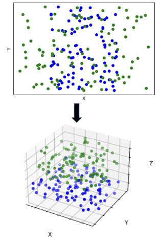
• A nonlinear SVC is used when the training data cannot be linearly separated
  • The classifier cannot be expressed as a linear function of independent variables
• It uses a nonlinear function, generally a polynomial equation with degree ≥ 2
  • Eg: y_i = f(x_i) = ax_i³ + bx_i² + cx_i + d
  • A nonlinear function is one where the output change nonlinearly with the input
• It uses the ‘kernel trick’ or kernel function to build the maximum-margin hyperplane
  • A kernel function transforms the data to a higher dimension feature space (Eg: 2D to 3D), to make it linearly separable by a hyperplane
  • Which is then transformed backed to the lower dimension with the linear separating hyperplane
  • Kernel functions can be Polynomial, Radial Basis, Gaussian, etc
  • kernel functions are generally distance weighted similarity functions (weighted sum, integral) which assign weights to the training data
  • They don’t explicitly calculate the dimension coordinates of the vectors (data points) in the feature space
• 

• A multiclass SVM classifier is used when the training data is to be separated into more than 2 classes (0,1,2,..,n)
• It transforms the multiclass classification problem into multiple binary classification problems
• It uses different strategies for building the multiclass classifier
  • ’one-vs-one’ – trains one classifier per pair of classes from the training data
  • The class with the most votes gets selected by the combined classifier
  • ‘one-vs-rest’ – trains one classifier per class, with the samples of that class labelled as +1 and all other samples as -1
  • For each classifier its class is fitted against all other classes
  • This is the preferred strategy for multi-class classifiers
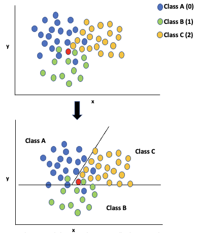
• Eg: In the given plot of training data with 3 classes (A,B,C or 0,1,2), assigning a class to the unlabeled data point (red dot) is not easy due to similarity to all 3
  • By applying multiclass SVC the training data can be separated into distinct classes by hyperplanes
  • The unlabeled data point (red) can now be correctly labelled with class C (2), being inside its boundary
• 

Naïve Bayes

• Use conditional probability models like Bayes theorem
  • It is the probability of an event occurring depending on the occurrence of prior related events
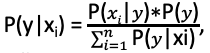
• For 2 events x and y, it states that P(y|x) = (P(x|y)∗P(y))/(P(x))  , where
• y – class variable (dependent), x – feature space (independent variables)
• It is also expressed as: Posterior probability = (Likelihood ∗ Prior probability) / Evidence
• If the feature space is partitioned into n mutually exclusive samples (x₁, x₂,…, x_n), then for any y, using law of total probability
• , where x_1,…, x_n is the independent variable feature space
• is constant being the input data (evidence)
• So, Bayes theorem becomes: P(y|x_i) ∝ P(x_i|y)∗P(y)
• Using joint probability and chain rule
  • P(x_i| y)∗P(y) = P(x₁,..,x_n, y) = P(x₁|x₂,..,x_n, y)*P(x₂|x_{1 ,}x₃,..,x_n, y)*…* P(x_n|x_{n-1 ,}y)*P(x_n|y)*P(y)

• Naïve Bayes makes the “naïve” assumption of conditional independence (no relationship) between every pair of features for a given a class variable
  • Normally there is some relationship (correlation) between different features in the training data
• Using the naïve assumption of conditional independence between x_1…n, the equation becomes
  • 
• The classifier then uses Maximum a Posteriori Probability (MAP) estimation to estimate the class label y ̂  for unlabelled data using the above equation
• MAP estimates the relative frequency of class y in the training set and selects the most likely value
• The classifier solves the equation:
• argmax (arguments of the maxima) is the subset of x for which y = f(x) is maximized
• Despite its oversimplified assumption, naïve bayes classifiers work quite well in many real-world applications like document classification and spam filtering
• They require a small amount of training data to estimate the necessary parameters
• They can be extremely fast compared to more sophisticated methods

• Different types of naïve bayes classifiers are dependent on the type of distribution they assume for P(xi|y )– Gaussian, Multinomial, Bernoulli
• Gaussian – Used for continuously distributed training data, as a Gaussian distribution, associated with each class
• Multinomial – Used for multinomially distributed data, feature count of discrete features, like word vector counts for text classification
• Bernoulli – Used for multivariate Bernoulli distributions, multiple binary valued features
  • It uses the occurrence count of binary features and used for short document classification

Ensembles (Random Forest, XGBoost)

• Are built using the same logic as in regression. Main difference is that for classification the algorithms generate discrete outputs (class labels)

Pipeline and GridSearchCV

• Now we will see how to use these libraries to build, optimize and evaluate multiple classification algorithms at once and then select the best one
• Pipeline combines data transformations and training multiple models into a sequence of steps
  • Grid search across entire hyperparameter grid to select the best combination for each model
  • Hyperparameters to be tuned for each model are setup as a predefined parameter array (grid)
• GridSearchCV performs k-fold cross-validation to train models on multiple variations of the training data of the sample in an iterative loop (k-folds, k-splits)
• The classification algorithms considered are
  • LogisticRegression
  • SVC
  • GaussianNB
  • KNeighborsClassifier
  • RandomForestClassifier
  • XGBClassifier
• A 10-fold cross-validation splitting strategy is used to ensure multiple variations of the training data are used (better data sampling)
• The results are better for all models
  • The hyper-tuned parameters can now be used for each model
• Logistic regression and SVC still give the best results compared to other models

Giving the code for Pipeline and GridSearchCV here as it shows how easy it is to try different classification models with hyperparameter tuning with just over 100 lines of code.

#Selecting the Best classifier with tuned hyperparameters using Pipeline and GridSearchCV

#Import libraries

import pandas as pd
from sklearn.linear_model import LogisticRegression
from sklearn.naive_bayes import GaussianNB
from sklearn.svm import SVC
from sklearn.neighbors import KNeighborsClassifier
from sklearn.ensemble import RandomForestClassifier
from xgboost import XGBClassifier
from sklearn.model_selection import train_test_split
from sklearn.preprocessing import StandardScaler #OneHotEncoder
from sklearn.metrics import confusion_matrix, ConfusionMatrixDisplay, classification_report, accuracy_score
from sklearn.pipeline import Pipeline
from sklearn.model_selection import GridSearchCV
import datetime
import warnings
warnings.filterwarnings(‘ignore’)

#Import the data

data = pd.read_csv(‘/Users/nitinsinghal/DataScienceCourse/Part1-MachineLearningDataAnalytics/Data/nbarookie5yrsinleague.csv’)

#view top 5 rows for basic EDA

print(data.head())

#Data wrangling to replace NaN with 0, drop duplicate rows

data.fillna(0, inplace=True)
data.drop_duplicates(inplace=True)

#Split the data into depdendent y and independent X variables

X = data.iloc[:, 1:-1].values
y = data.iloc[:, -1:].values

#As y is a column vector and the algorithm expects a 1D array (n,) we need to reshape the array using ravel()

y = y.ravel()

#Encode the catgorical data (text or non-numeric data needs to be converted into a binary matrix of ‘n’ categories)

encoder = OneHotEncoder(drop=’first’, sparse=False, handle_unknown=’error’)

X_encoded = encoder.fit_transform(X)

#Split the data into training and test set

X_train, X_test, y_train, y_test = train_test_split(X, y, test_size = 0.25)

#Scale (Standardize) the X values as large values can skew the results by giving them higher weights

scaler = StandardScaler()
X_train = scaler.fit_transform(X_train)
X_test = scaler.transform(X_test)

# Create the pipeline to run gridsearchcv for best classifier and hyperparameters

pipe_lrc = Pipeline([(‘clf’, LogisticRegression())])

pipe_svc = Pipeline([(‘clf’, SVC())])

pipe_gnb = Pipeline([(‘clf’, GaussianNB())])

pipe_knn = Pipeline([(‘clf’, KNeighborsClassifier())])

pipe_rfc = Pipeline([(‘clf’, RandomForestClassifier())])

pipe_xgb = Pipeline([(‘clf’, XGBClassifier())])

#Set grid search params

grid_params_lrc = [{‘clf__solver’ : [‘lbfgs’, ‘liblinear’],
‘clf__C’ : [0.001,0.01]}]

grid_params_svc = [{‘clf__kernel’ : [‘linear’,’rbf’],
‘clf__C’ : [0.1,0.5]}]

grid_params_gnb = [{}]

grid_params_knn = [{‘clf__n_neighbors’ : [20,50],
‘clf__weights’ : [‘uniform’, ‘distance’]}]

grid_params_rfc = [{‘clf__n_estimators’ : [200],
‘clf__min_samples_split’ : [2],
‘clf__min_samples_leaf’ : [1,2],
‘clf__max_features’ : [‘auto’,’log2′],
‘clf__random_state’ : [42]}]

grid_params_xgb = [{‘clf__objective’ : [‘binary:logitraw’,’binary:hinge’],
‘clf__lambda’ : [1,2]}]

#Create grid search

gs_lrc = GridSearchCV(estimator=pipe_lrc,
param_grid=grid_params_lrc,
scoring=’accuracy’,
cv=10,
n_jobs=-1)

gs_svc = GridSearchCV(estimator=pipe_svc,
param_grid=grid_params_svc,
scoring=’accuracy’,
cv=10,
n_jobs=-1)

gs_gnb = GridSearchCV(estimator=pipe_gnb,
param_grid=grid_params_gnb,
scoring=’accuracy’,
cv=10,
n_jobs=-1)

gs_knn = GridSearchCV(estimator=pipe_knn,
param_grid=grid_params_knn,
scoring=’accuracy’,
cv=10,
n_jobs=-1)

gs_rfc = GridSearchCV(estimator=pipe_rfc,
param_grid=grid_params_rfc,
scoring=’accuracy’,
cv=10,
n_jobs=-1)

gs_xgb = GridSearchCV(estimator=pipe_xgb,
param_grid=grid_params_xgb,
scoring=’accuracy’,
cv=10,
n_jobs=-1)

#List of grid pipelines

grids = [gs_lrc, gs_svc, gs_gnb, gs_knn, gs_rfc, gs_xgb]

#Grid dictionary for pipeline/estimator

grid_dict = {0:’LogisticRegressionClassifier’, 1: ‘SupportVectorClassifier’, 2:’GaussianNaiveBayesClassifier’, 3:’KNNClassifier’,
4:’RandomForestClassifier’, 5:’XGBoostClassifier’}

#Fit the pipeline of estimators using gridsearchcv

print(‘Fitting the gridsearchcv to pipeline of estimators…’)
resulterrorgrid = {}

for gsid,gs in enumerate(grids):
print(‘\nEstimator: %s. Start time: %s’ %(grid_dict[gsid], datetime.datetime.now()))
gs.fit(X_train, y_train)
print(‘\n Best score : %.5f’ % gs.best_score_)
print(‘\n Best grid params: %s’ % gs.best_params_)
y_pred = gs.predict(X_test)
# Accuracy score
accscore = accuracy_score(y_test, y_pred)
print(‘accuracy_score: ‘, accscore)
# Accuracy metrics
accmetrics = classification_report(y_test, y_pred)
print(‘classification_report: \n’, accmetrics)
# Calculate and plot the confusion matrix for predicted vs test class labels
cm = confusion_matrix(y_test, y_pred)
disp = ConfusionMatrixDisplay(confusion_matrix=cm)
disp.plot()
resulterrorgrid[grid_dict[gsid]+’best_params’] = gs.best_params
resulterrorgrid[grid_dict[gsid]+’best_score’] = gs.best_score
resulterrorgrid[grid_dict[gsid]+’_accscore’] = accscore
resulterrorgrid[grid_dict[gsid]+’_accmetrics’] = accmetrics
resulterrorgrid[grid_dict[gsid]+’_cm’] = cm

print(‘result grid: ‘, resulterrorgrid)