Clustering- Unsupervised learning- Types, Metrics

This article will discuss the basic theory and relevant code examples for different clustering algorithms.

Code for different algorithms and data used are given in github.

Note – Make sure to point the code to the right directory in your setup

https://github.com/datawisdomx/DataScienceCourse/tree/main/Part1-MachineLearningandDataAnalytics/Examples/Chapter10_Clustering

https://github.com/datawisdomx/DataScienceCourse/tree/main/Part1-MachineLearningandDataAnalytics/Data

Clustering – Unsupervised learning algorithm

• It uses unlabeled training data X to separate it into y clusters (classes) using some similarity measure (distance, density, etc)
  • Data points similar (close) to each other are assigned to one cluster
  • It is unlike supervised algorithms that require labeled data to learn from in order to build models to make predictions
• It is a multi-objective optimization algorithm that uses an iterative process to find the best fit clusters for the training data
• A new unlabeled observation can then be assigned to the right cluster based on the distance metric used
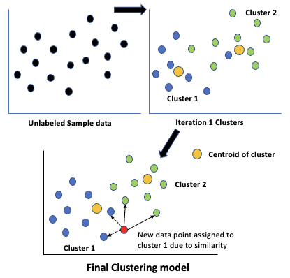
• In the figure shown, the clustering algorithm starts with the unlabeled sample data and performs multiple iterations of
  • Splitting the data into target number of clusters and calculating their centroid
  • In the next iteration it reassigns the data to clusters using the previous iterations centroids and calculates the new centroid, repeating this till an optimal value is reached
  • The splitting, no of iterations, centroid calculation, etc depend on the algorithm used and its defined parameters
  • No of clusters are generally user defined or estimated by the algorithm

Metrics:

• Silhouette Coefficient – defines how well defined and dense the clusters are. Useful when actual y values are unknown. Between (-1,1). Closer to 1 better
• Adjusted Rand index – proportional to the number of sample pairs with same labels for predicted and actual y labels. Between (0,1). Closer to 1 better
• Homogeneity – each cluster contains only members of a single class. Between (0,1). Closer to 1 better
• Completeness – all members of a given class are assigned to the same cluster. Between (0,1). Closer to 1 better
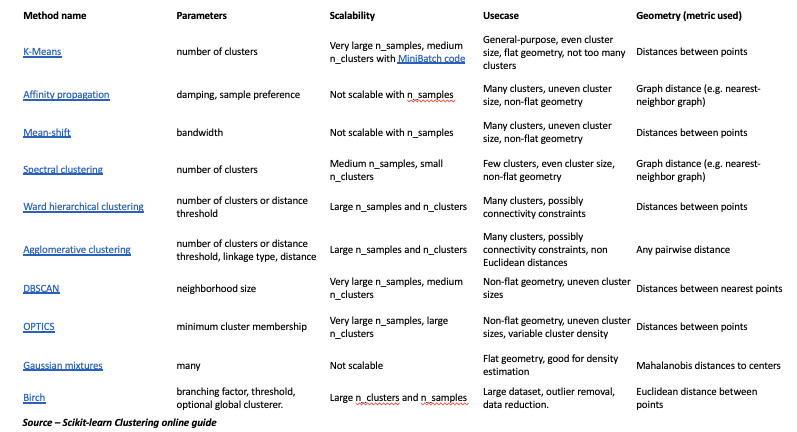
• Different clustering algorithms depend on the type of distance metric used. Some common one’s are discussed Useful website – https://scikit-learn.org/stable/modules/clustering.html

K-Means

• Centroid based K-Means clustering algorithm separates the n samples of X into k clusters by minimizing the squared distance of the data point from the cluster mean C (centroid)
• Centroids are selected so that the within-cluster-sum-of-squares WCSS (inertia) is minimized
• The equation to be solved is 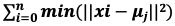. μ_j ∈ C, is the mean of each cluster (j = 1 to k)
• The algorithm works by first randomly initializing k, then repeats the below steps till the threshold is reached
  • Assigns each sample x_i to the nearest centroid μ_j
  • It then creates new centroids by taking the mean of samples assigned to each previous centroid
  • Difference between the mean of the old and new centroids is compared to the threshold
  • These 3 steps are repeated till the threshold is reached
• As k is randomly fixed at the start, it is a drawback as the algorithm has to be repeated for different values
• To over come this random initialization issue the Elbow method and K-Means++ initialization are used
• The Elbow method gives a better initial value for k, by plotting the explained variance as a function of the no of clusters
  • The ‘elbow’ or ‘knee’ of the curve acts as the cut-off point for k for diminishing returns
  • The point where adding more clusters does not improve the model, cost vs benefit)
• K-means++ initialization further improves the results by initializing the centroids to be distant from each other
• K means algorithms assume that the clusters are convex shaped (outward curve, all parts pointing inwards. Eg: rugby ball)

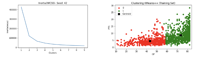
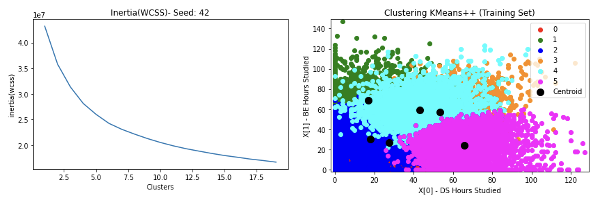
• The code for plotting the elbow curve to determine initial k is given in the example
  • It is determined by using the inertia_ attribute of the model
  • It is the Sum of squared distances of samples to their closest cluster centre (WCSS)
• Results NBA rookie stats to predict if a player will last 5 years in league as 2 clusters are given below

• Results for Kaggle Tortuga Code dataset to predict different students’ developer category as 6 clusters are given below

Hierarchical

• Connectivity based Hierarchical clustering algorithms build nested clusters by merging or splitting them successively by minimizing a linkage (distance) criteria
  • Observations closer to each other (distance) can be connected to form a cluster
• They can be agglomerative or divisive
  • Agglomerative algorithms use a bottom up approach starting with each sample observation X as a cluster and aggregates (merges) them successively into clusters
  • Divisive use a top down approach starting with the entire sample as a cluster and successively dividing it into clusters
• It is represented as a hierarchical tree (dendrogram)
  • Root is cluster of all samples and leaves are clusters of individual samples
• Different linkage criteria’s are:
  • Single – minimizes distance between closest observations of pairs of clusters
  • Average – minimizes average distance between all observations of pairs of clusters
  • Complete (Maximum) –  minimizes the maximum distance between observations of pairs of clusters
  • Ward – minimizes the sum of squared differences within all clusters. Minimizes variance. Similar to k-means
• Single linkage while being the worst hierarchical strategy, works well for large datasets and can be computed efficiently

DBSCAN

• Density based clustering algorithms define clusters as areas of high density separated by areas of low density
  • A cluster is a set of core samples close to each other (areas of high density) and a set of non-core samples close to a core sample (neighbors) but are not core samples themselves
  • The closeness is calculated using a distance metric
• DBSCAN (Density-Based Spatial Clustering of Applications with Noise) is a popular density based algorithm
  • It builds clusters using 2 parameters that define density
  • min_samples – minimum no of samples required in a neighborhood for a core sample
  • eps – maximum distance between two samples to be considered as each others’ neighbors
  • Higher min_samples or lower eps indicates higher density to form a cluster
• Density based clusters can be of any shape (unlike k-means convex shape)

Gaussian Mixture Model

• Distribution based clustering algorithms build clusters with samples belonging to the same distribution
• Gaussian Mixture Model (GMM) is a popular method within them
• GMM is a probabilistic model that assumes that all data points are generated from a mixture of finite Gaussian distributions (normal distribution) with unknown parameters
• It implements the Expectation-Maximization algorithm, which finds the maximum-likelihood estimates of unknown parameters of the model which depends on latent variables (inferred from observed samples)
• They suffer from limitations like scalability

The results of the different algorithms show that KMeans gives the best results

• It is more widely used and has better interpretability

Plotting in higher dimensions (above 3D) is difficult so dimension reduction techniques like LDA and PCA can be used